Heterogeneous canopies with anisotropic background
RAMI IV phase
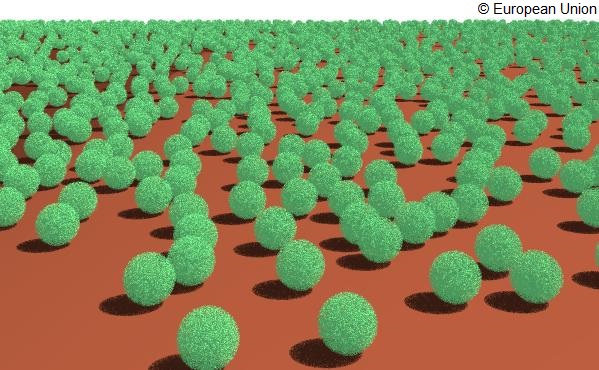
This set of experiments is suggested to simulate the radiative transfer regime in the red and near infra-red spectral bands for heterogeneous leaf canopies composed of a large number of identical, non-overlapping spherical objects - representing the individual plant crowns - located over and only partially covering a NON-LAMBERTIAN horizontal plane standing for the underlying background surface. These spherical objects have a radius of 0.5m and their centers are located 0.51 ± 0.0001 meters above the background plane (random height distribution) to yield a maximum canopy height of ~1.01m. To address the needs of different RT models, both a statistical scene description, as well as a file with the exact coordinates of every single scatterer in the canopy are provided.
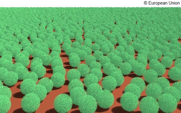
Two different fractional coverages (i.e., number of spheres per scene) are proposed: medium=0.2 and dense=0.4 coverages. Each individual sphere contains a 'cloud' of oriented finite-sized particles representing the foliage.
The leaf area index (LAI) of a single sphere (LAI = area of leaves ⁄ maximum cross section of sphere) is fixed and amounts to 5.0 [m² ⁄ m²]. Within a given sphere the Bi-Lambertian foliage elements are characterized by specified radiative properties (reflectance, transmittance) defined separately for both the visible and near-infrared spectral domains. The orientation of the normals of the foliage elements (scatterers) follows a uniform (or what is sometimes called a spherical) distribution function, i.e., the probability to be intercepted by a leaf is independent of the direction of travel of the radiation (see the definitions page). The BRF of the anisotropically scattering background (which is intended to represent snow, bare soil and understorey vegetation conditions, respectively) is expressed with the parametric RPV model. Participants who wish to fit their own anisotropic background model to the RPV-simulated BRF data should inform the RAMI coordinators of this via the report files.
The figure exhibits graphical representations of the sparse scene.
The figure exhibits graphical representations of the dense scene.
Description for SPARSE scene
The tables below provide the details required to build and run a RT model on the sparse scene with anisotropic scattering properties of the underlying background (snow, vegetation, soil).
Scene properties:
( X × Y × Z)
101.0 × 101.0 × 1.01 [m × m × m]
(Xmin, Ymin, Zmin)
−50.5, −50.5, 0.0 [m, m, m]
(Xmax, Ymax, Zmax)
+50.5, +50.5, 1.0101 [m, m, m]
Scatterer shape
Disc of negligible thickness
Scatterer radius
0.005 [m]
LAI of individual sphere
5.0
Scatterer normal distribution
Uniform
Foliage scattering law
Bi-Lambertian
Number of spheres
2547
Fractional scene area coverage of spheres
0.1961
Sphere radius
0.5 [m]
Minimum sphere center height
0.5099 [m]
Maximum sphere center height
0.5101 [m]
background BRF pattern
Non-Lambertian (see tables below)
where the Leaf Area Index (LAI) is calculated as follows:
LAI = (# of leaves × one-sided area of single leaf) ⁄ (π × square of the radius of sphere)
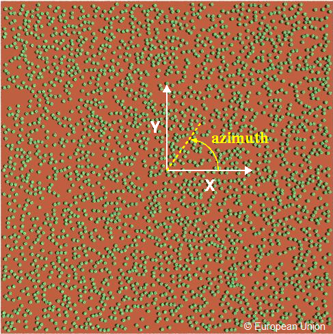
The figure exhibits top sparse scene representation.
An ASCII file with the radius (R), centre coordinates (Xc,Yc,Zc), and direction cosines (Dx,Dy,Dz) of every single leaf in a spherical volumes centered at 0,0,0 can be found here. This file (is ~ 2.7 Mbytes and) contains 49999 lines of format R Xc Yc Zc Dx Dy Dz that may serve as input to your scene creation process (provided that you are able to create multiple instances of its content, each one of which is then translated to the actual locations of the sphere centers in the scene. The coordinates (X, Y, Z) of the various sphere centers for the medium dense scene can be found here.
The tables below provide detailed information regarding the illumination conditions and spectral properties of the foliage and background constituents of the sparse canopy scenarios.
Every table is preceeded by the corresponding experiment identifier tag <EXP> that is needed in the naming of the various measurement results files (see file naming and formatting conventions). Two spectral bands (red and NIR) and two illumination conditions (direct only with SZA=20° and 50°) are proposed for three different background anisotropy scenarios, referred to as HET10, HET11 and HET12 in the tables below. The difference between experiments HET10, HET11 and HET12 thus lies only in the BRF of the anisotropically scattering background (assumed to be reminiscent of snow, bare soil, and understorey vegetation).
The background BRF is described by the three parameter of the RPV model.
Description for DENSE scene
The tables below provide the details required to build and run a RT model on the dense scene with anisotropic scattering properties of the underlying background (snow, vegetation, soil).
Scene properties:
( X × Y × Z)
101.0 × 101.0 × 1.01 [m × m × m]
(Xmin, Ymin, Zmin)
−50.5, −50.5, 0.0 [m, m, m]
(Xmax, Ymax, Zmax)
+50.5, +50.5, 1.0101 [m, m, m]
Scatterer shape
Disc of negligible thickness
Scatterer radius
0.005 [m]
LAI of individual sphere
5.0
Scatterer normal distribution
Uniform
Foliage scattering law
Bi-Lambertian
Number of spheres
5093
Fractional scene area coverage of spheres
0.3921
Sphere radius
0.5 [m]
Minimum sphere center height
0.5099 [m]
Maximum sphere center height
0.5101 [m]
background BRF pattern
Non-Lambertian (see tables below)
where the Leaf Area Index (LAI) is calculated as follows:
LAI = (# of leaves × one-sided area of single leaf) ⁄ (π × square of the radius of sphere)
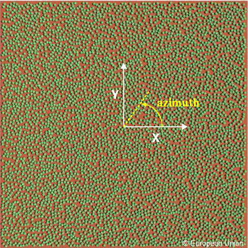
The figure exhibits top dense scene representation.
An ASCII file with the radius (R), centre coordinates (Xc,Yc,Zc), and direction cosines (Dx,Dy,Dz) of every single leaf in a spherical volumes centered at 0,0,0 can be found here. This file (is ~ 2.7 Mbytes and) contains 49999 lines of format R Xc Yc Zc Dx Dy Dz that may serve as input to your scene creation process (provided that you are able to create multiple instances of its content, each one of which is then translated to the actual locations of the sphere centers in the scene. The coordinates (X, Y, Z) of the various sphere centers for the medium dense scene can be found here.
The tables below provide detailed information regarding the illumination conditions and spectral properties of the foliage and background constituents of the sparse canopy scenarios.
Every table is preceeded by the corresponding experiment identifier tag <EXP> that is needed in the naming of the various measurement results files (see file naming and formatting conventions). Two spectral bands (red and NIR) and two illumination conditions (direct only with SZA=20° and 50°) are proposed for three different background anisotropy scenarios, referred to as HET20, HET21 and HET22 in the tables below. The difference between experiments HET20, HET21 and HET22 thus lies only in the BRF of the anisotropically scattering background (assumed to be reminiscent of snow, bare soil, and understorey vegetation).
The background BRF is described by the three parameter of the RPV model.