European Commission - RAMI website

This page provides descriptions of the architectural, spectral and illumination related properties of a 124 year old Pinus sylvestris stand located at 58° 18′ 47.13″ N 27° 17′ 48.23″ E, The stand was inventoried in the summer 2007 by Andres Kuusk, Joel Kuusk, Mait Lang, Tõnu Lükk, Matti Mõttus, Tiit Nilson, Miina Rautiainen, and Alo Eenmäe of the Tartu Observatory, in Tõravere, Estonia as well as the Estonian University of Life Sciences, Tartu, Estonia.

Potential RAMI participants thus are to treat the information presented on this page as actual 'inventory data', that is, they should identify/extract those parameters and characteristics that are required as input to their canopy reflectance models.

In some cases this may mean that simplifications have to be made to the available information, or, that parts of the available information cannot be - or have to be modified before being - exploited with a given radiative transfer model. Whatever the case may be, all potential RAMI participants should mimic the standard practices that they use when matching actual field measurements to the required set(s) of input parameters for their model(s). If this means that you need more information than provided, please do not hesitate in contacting us. Last but not least, for those 3D models capable of maintaining architectural fidelity down to the individual shoot and branch level a series of ASCII (text) files containing the Cartesian coordinates of various geometric primitives (triangles, spheres and cylinders) and their transformations will be given.

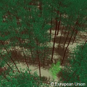
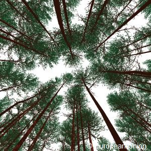
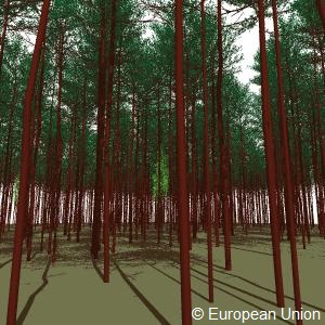
Figure 1: Järvselja Pine Stand (Summer) scene description.

Architectural information

The Järvselja Scots Pine forest inventory was carried out over a 100×100 m² area placing the origin of the coordinate system at its south-western end. In order to include also the tree crowns of the inventoried tree locations within the RAMI Scots Pine Summer stand representation it was necessary to expand the scene area slightly beyond one hectare. Maintaining the origin of the tree location coordinate system thus resulted in some negative x,y values in the table below. Overall architectural characteristics of the scene are thus as follows:

Scene dimensions:( X × Y × Z)	105.932 × 106.118 × 18.560 [m × m × m]
(Xmin, Ymin, Zmin)	−2.773, −3.623, 0.0 [m, m, m]
(Xmax, Ymax, Zmax)	103.159, 102.495, 18.560 [m, m, m]
Number of trees in scene	1120 (1114 pine, 6 birch)
Leaf Area Index of scene*	2.3020 (2.2881 pine, 0.0139 birch)
Fractional scene coverage**	0.406

Table 1: Architectural information

*The LAI of the pine trees is computed using half the total area of the needles in a shoot.

**The fractional cover is defined as 1 - direct transmission at zero solar zenith angle.

Foliage structure

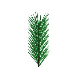
The table below provides the structural characteristics of the Scots Pine shoots (left) and the birch leaves (right).
Individual shoots of the Scots Pine trees are generated in using most of the properties presented in Table 1 of Smolander et al., 2003 (RSE).
The shape of individual birch tree leaves is approximated from photographs as depicted in the right hand picture.
RT models capable of representing the architecture of individual foliage elements with a series of geometric primitives (triangle, sphere, cylinder) may want to use the information provided in the ASCII (text) files accessible from the last row in each table below.

number of needles	190
total needle area*	122.98 cm^²
needle length	2.85 cm
needle diameter	0.092 cm
angle between twig and needle	40.5°
fascicle angle	0 - 27.7°
twig length	7.7 cm
twig diameter	0.3 cm
structural description file (geometric primitives)	click here

Table 2: Scots pine shoot foliage structure.

leaf length (excluding twig)	6.92 cm
Max. radial leaf extension away from the twig-to-tip axis	2.58 cm
one sided leaf area	20.7 cm^²
twig length	0.5 cm
twig diameter	0.3 cm
leaf curl	none
structural description file (triangle mesh)	click here

Table 3: Birch tree leaf foliage structure.

* This total needle area value arises if the needles are represented as elongated spheres (as is the case in the ASCII file accessible via the link in the last row of the above left-side table). If individual needles are represented as cylinders (with discs as endcaps) then the total needle area of the shoot is 159.03 cm². The number of shoots per pine tree should be adjusted accordingly.

Tree structure

The Järvselja Scots Pine forest is generated on the basis of 11 individual tree representations. Ten of these pertain to the Scots pine (Pinus Sylvestris) species and one refers to Birch (Betula Pendula). The table below provides an overview of some structural characteristics of these 11 tree representations. For those RT models capable of representing the 3D architecture of a given tree through a series of geometric primitives the last lines of this table contain links to data files with detailed specifications of the foliage and wood structural properties of the Järvselja Scots Pine forest (summer) trees.

tree identifier		PISY1	PISY2	PISY3	PISY4	PISY5	PISY6	PISY7	PISY8	PISY9	PISY10	BEPE
tree height [m]		16.58	17.40	17.97	18.56	10.45	10.21	11.78	13.18	14.28	15.54	16.19
Foliage normal distribution: zenith angle=		graph data	graph data	graph data	graph data	graph data	graph data	graph data	graph data	graph data	graph data	graph data
Foliage normal distribution: azimuth angle=		graph data	graph data	graph data	graph data	graph data	graph data	graph data	graph data	graph data	graph data	graph data
height to live/green crown [m]		9.01	9.09	11.26	11.08	11.49	11.48	11.59	11.70	11.97	11.87	3.06
crown radiusx	mean [m]	0.96	1.11	1.16	1.42	0.62	0.15	0.31	0.47	0.51	0.73	0.95
	maximum [m]	2.24	2.51	2.75	3.70	1.43	0.49	0.75	1.19	1.16	1.72	2.19
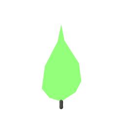
	picture	picture	picture	picture	picture	picture	picture	picture	picture	picture	picture	picture
vertical profile of crown radii* [m]		graph data	graph data	graph data	graph data	graph data	graph data	graph data	graph data	graph data	graph data	graph data
half-total foliage area of tree# [m^²]		1.2975	2.8163	5.4113	10.2691	15.3667	23.8526	31.127	39.9818	58.9458	79.0104	8.7978
vertical profile of leaf area° [m]		graph data	graph data	graph data	graph data	graph data	graph data	graph data	graph data	graph data	graph data	graph data
trunk DBH+ [cm]		6.1	8.7	11.5	13.3	15.1	18.0	20.5	22.6	27.3	31.8	5.4
total wood area of tree [m^²]		1.5598	2.6613	5.5951	5.7453	16.4526	22.5192	23.6616	30.3588	47.0282	79.8664	3.1673
vertical profile of wood area° [m^²]		graph data	graph data	graph data	graph data	graph data	graph data	graph data	graph data	graph data	graph data	graph data
dead branch number		9	3	36	4	13	8	8	8	0	0	0
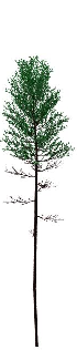
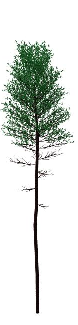
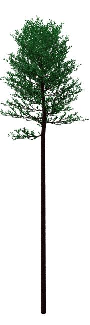
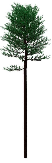
tree shape image
Foliage		file	file	file	file	file	file	file	file	file	file	file
Stems		file	file	file	file	file	file	file	file	file	file	file
Branches		file	file	file	file	file	file	file	file	file	file	file

Table 4: tree structure.

=: for shoots the zenith angle of the foliage normal is defined as the angle between the vertical and the normal of the inner/main twig of the shoot (for a shoot axis aligned along the z-axis the normal was arbitrarily chosen to lie along the y-axis). Rather than spanning the full range of possible zenith angles (i.e., from 0 to 180°) as could be expected for non-flat asymmetric objects, it was chosen to follow the convention of foliage normals pointing only into the upper hemisphere. This is because RAMI participants, that make use of this foliage normal distribution information, will in all likelihood have models where scatterers are represented as flat (disc or equilateral triangle shaped) objects. However, should your model require a description of the foliage normal zenith angle distribution up to 180° then please do not hesitate in contacting us and we will provide this information to you. For both the zenith and azimuth angle distributions the 'graph' link shows an image of the normalised foliage normal distribution versus zenith (or azimuth) angle of the foliage normal. The 'data' files for the zenith and azimuth angle distribution have three columns indicating

the upper value of the zenith (or azimuth) angle in a given bin,
the fraction of foliage area having a normal in this zenith (or azimuth) angle range,
and the fraction of wood area having a normal that falls in this zenith (or azimuth) angle range. Bin angle widths were chosen to be 5° and 10° for zenith and azimuth angles, respectively.

x: the crown radius of actual trees is varying with azimuth angle. This can be seen in the various pictures showing a perspective-free nadir view of a given tree located at x=0,y=0 (concentric circles indicate the distance from the origin in steps of 0.25m). The mean and maximum values were computed from the triangle objects making up the 3D trees depicted in the picture in the the fourth-last row of each table column.

*: the graphs show the maximum radial distance of foliage elements in a given height interval plotted against the upper height level of that height interval. The data files have five columns: lower height of bin (m) upper height of bin (m) minimum_radial-distance_of_foliage-in-units-of-m maximum_radial-distance_of_foliage-in-units-of-m. mean_radial-distance_of_foliage-in-units-of-m

#: this value corresponds to the one-sided leaf area for flat leaves. For Scots pine trees it corresponds to the sum of the (maximum) silhouettes of all the individual needles in the tree (i.e., half the total needle area per tree).

°: the data files have 3 columns: lower height of bin (m) upper height of bin (m) area of wood or foliage (m²).

+: his is the nominal value derived from the inventory data for a tree of this height. The actual value of the tree representations provided in the ASCII files at the bottom of this table might be slightly different.

Stand structure

The Järvselja Scots Pine forest is composed of 1120 individual trees. The following table indicates how these trees are distributed among the above tree classes and specifies their respective x,y locations of the tree centers of each tree class in the forest stand. The last row of this table contains an ASCII file with tree rotation and translation information for those RT models capable of ingesting the detailed 3D architecture of the tree models specified in the previous section.

tree identifier	PISY1	PISY2	PISY3	PISY4	PISY5	PISY6	PISY7	PISY8	PISY9	PISY10	BEPE
tree number per class	8	29	100	149	220	219	193	147	40	9	6
x,y coordinates of tree centers [m,m]	data	data	data	data	data	data	data	data	data	data	data
tree rotations and translation (ASCII file)x	data	data	data	data	data	data	data	data	data	data	data

Table 5: stand structure.

x: these files contain pseudo code to rotate individual trees around their z axis and translate them from the origin to the x,y locations specified in the data files of the previous row of this table. Positive rotation angles in these files indicate that when looking down from the positive Z axis towards the origin of the coordinate system a counterclockwise rotation will result in moving the positive x axis towards the positive y axis. The angle of rotation is in the 7th column of these data files (starting the count from 1).

RAMI participants with 3D RT models capable of representing objects using geometric primitives can download a single compressed ZIP archive with all the tree architectural ASCII information that is listed in the above tables by clicking HERE.

Note: The size of the compressed archive is about 9.3 megabytes. It contains 46 ASCII files and can be unzipped using 'WINZIP' on windows or 'unzip' on linux/unix operating systems.

Beware that the inflated archive will take up 65.9 Megabytes of storage.

Figure 4: Tree species and locations for the Järvselja Scots pine (summer) stand. The origin of the coordinate system is in the lower left hand side corner of the image.

Spectral canopy characteristics

All of the foliage wood and background components in the Järvselja pinestand (summer) scene feature LAMBERTIAN scattering properties. The tables below contain the magnitudes of the reflectance and transmission characteristics of the various canopy components for fourteen different spectral bands. The experimental identifier for the Järvselja Pine Stand (Summer) scene is given by HET07_JPS_SUM_BBB_zZZaAAA where BBB is one of the spectral bands of RAMI-V (O03,O04,O06,O08,O10,O11,O12,M08,O17,MD5,M11,MD7,M12,GED). An ASCII (text) file summarising all of this information can be found here.

Illumination characteristics

The illumination conditions are very likely dependent on the kind of measurement in RAMI-V more than in previous RAMI phases. For brf*, dhr, fabs*, ftran* measurements, except brf_sat, the illumination were listed in the description of measure brfpp, and duplicated in other measure description pages. For these geometries the tag will be _zZZaAAA_ with ZZ and AAA defining $\theta_i$ and $\phi_i$, respectively. In addition, diffuse isotropic illumination is foreseen for bhr, fabs*, ftran* measures (geometry tag will then be _DIFFUSE_). lidar* like measurements and thp illumination are described in the relevant measure description pages, and are the same for all scenes for which they are foreseen.

Scene	Site	Jan	Apr	Jul
HET07_JPS_SUM	Järvselja		_z56a153_	_z41a147_

Table 6: Illumination conditions.