
HET50_SAV_PRE
New additional files has been released for this test-case: see News section.
Pre-fire models of a two-layer savanna heterogeneous system were established including an overstory (tree) and an understory (grass) layer. The models were developed from detailed field measurements of structural and radiometric properties made at experimental burn plots with varying canopy cover in the Kruger National Park, South Africa. Skukuza (25.1097 S, 31.4172E) and Pretoriuskop (25.1639 S, 31.234E), both sited at long-term fire ecology experimental plots in the KNP [van Wilgen et al.,2004].
At each plot a range of pre-fire structural and radiometric measurements of the tree-dominated overstory and grass understory were made to enable the development and testing of the 3D models.
The Skukuza plots are dominated by shallow rooted deciduous Combretum species, in particular Combretum apiculatum (Red Bushwillow), Combretum hereroensis (Russet Bushwillow) and Combretum zeyheri (Mixed Bushwillow). These trees make up a significant part of the total biomass, even though many of them lie horizontally after being felled by young elephants.
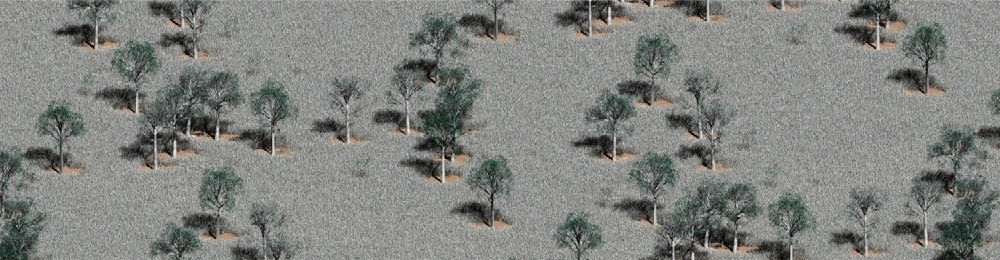
Using the information from the field measurements, 3D tree and grass models were generated to produce 3D savanna scene models of 100×100 m extent. 3D model canopies covering a range of vegetation density (tree and grass LAI) were produced to match the range of field measurements, over a soil understory using measured soil reflectance properties. In all cases where plant models re located within the scenes, a uniform random distribution is used.
For the Combretum, Sclerocarya and Terminaliastructure, Onyx-TREE © software was used. This software has been used to simulate the structure of deciduous broadleaf canopies for simulation of various remote sensing signals [Disney et al.,2009, IEEE, Disney et al.,2010, RSE]. Ten individual Combretum and Sclerocarya trees were generated, spanning the observed range of height and crown size [provide model for all trees].
Backfires were lit on the downwind side of the plots first, before headfireswere lit on the upwind side some 10–15 minutes later. Areas remaining unburned were relit within 30 minutes. Pre-fire fuel load measurements showed that around 90-95% of the standing grass and 96% of the litter was burned in the Skukuza plots, and 100% of the grass and litter were burned in the Pretoriuskop plots. In both cases the overstory was not affected, a situation common to a range of arid African savanna fires.
3D tree structure was developed using OnyxTREE© software, parameterised using the detailed measurements of tree height, DBH, and crown size made in the field. These measurements were used to develop trees in leaf-on and leaf-off conditions, for the dominant species at the sites. To generate plot-sized scenes (100x100m) trees are arranged randomly within a given plot, according to a predefined planting density (and standing, falling), determined from the field observations.
3D grass structure: due to large amount of understorey grass cover, cylinders of varying lengths have been used to represent the grass objects, to mantain efficiency of calculation. This can lead to possible under-representation of forward scattering (transmittance) through the cylinders when hit by a photon.
Figure 2 shows examples of the key 3D scene model components.
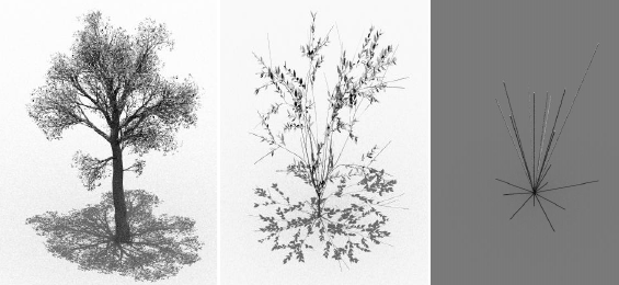
The range of individual plant models used to buildbuilt the savanna 3D scene is summarised as follows. The individual plants comprise:
The 3D models of trees and grass plants used in this scene (Table 1, Table 2, Table 3) are released as Waveform OBJ files and Rayshade format. The former are suitable to be imported in 3D graphics programs such as Blender for the tree rendering and conversion to other formats suitable to be imported in RTM models (File -> export). The rayshade format is a more descriptive format which helps to build a scene with the use of individual primitives (in particular here triangles and cylinders are used for leaf and trunk/branch representation).
The whole scene consists of clones of different types of trees and grass plants over a 1ha squared area. Figure 3 shows the distribution of the different models over the 1ha scene.
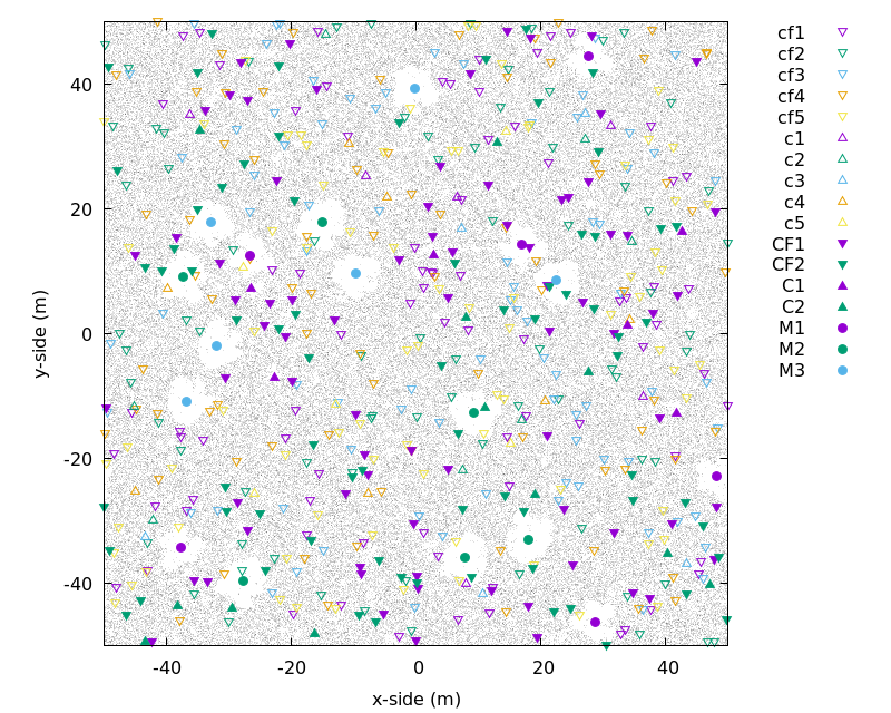
The coordinates of grass and tree models are given in grass.all.xyz file and trees.all.xyz, respectively. Figure 3 illustrates the position of each tree model and grass distribution. Grass does not grow below Merula trees. The columns content of coordinates .xyz files are:
| Model | Stand version | Instances | Flat versions | Istances | Render (stand | |
|---|---|---|---|---|---|---|
| version only) | ||||||
| combretum leafoff | 1 | stand obj | 6 | flat obj | 77 |  |
| 2 | stand obj | 7 | flat obj | 76 |  |
|
| 3 | stand obj | 5 | flat obj | 78 |  |
|
| 4 | stand obj | 7 | flat obj | 76 |  |
|
| 5 | stand obj | 5 | flat obj | 78 |  |
| Rayshade | Wavefront | Instances | TLA | NL | CR (m) | Render | ||
|---|---|---|---|---|---|---|---|---|
| .def | .obj | ($m^2$) | ||||||
| combretum leafon |
1 | def | obj | 6 | 1.919 | 1622 | 1.575 |  |
| 2 | def | obj | 12 | 0.024 | 17 | 0.940 |  |
|
| combretum leafon flat |
1 | def | obj | 77 | -- | -- | -- |  |
| 2 | def | obj | 71 | 0.024 | 17 | 0.940 |  |
|
| merula | 1 | def | obj | 6 | 15.076 | 5202 | 4.227 |  |
| 2 | def | obj | 6 | 52.701 | 18228 | 4.553 |  |
|
| 3 | def | obj | 6 | 57.705 | 19953 | 4.310 |  |
|
| All | // | def | obj | 178 | // | // | // | // |
Ten different models (grass.[0-9].obj), defined by sets of cylinders, represent grass plants. The models are then randomly distributed over the entire scene (x,y,z=0), accordingly to grass.[0-9].xyz or grass.all.xyz files. For each model, approximately 20,000 instances should be generated for a total number of grass plants of 200,000 over the entire 1 ha scene. Table 3 contains the link to the 10 different grass plant definitions (rayshade grass.#.def or wavefront grass.#.obj) and their position in the scenes (.xyz files). They are released in different formats for users convenience. For the format of these files please refer to the "notes on the file formats" section of the Wytham Wood scene description scene. In addition to the files defining individual plants, a set of standard wavefront files has been created by cloning each the individual plant accordingly to its coordinates and exporting the result as a triangular mesh. They can be promptly ingested by Wavefront file readers (e.g. Blender, Windows Print 3D, ...).
Users can contact the project leader for further information, scene bugs, suggestion of additional data formats.
| Model | Rayshade | Modified | Coords | N instances | Inclusive | Blender |
|---|---|---|---|---|---|---|
| wavefront | ||||||
| .def model | .obj model | Wavefront | Render | |||
| description | (Librat) | (>100MB) | (png) | |||
| 0 | grass.0 | grass.0 | grass.0 | 20105 | na |  |
| 1 | grass.1 | grass.1 | grass.1 | 20003 | na |  |
| 2 | grass.2 | grass.2 | grass.2 | 19813 | na |  |
| 3 | grass.3 | grass.3 | grass.3 | 20035 | na |  |
| 4 | grass.4 | grass.4 | grass.4 | 20146 | na |  |
| 5 | grass.5 | grass.5 | grass.5 | 19937 | na |  |
| 6 | grass.6 | grass.6 | grass.6 | 19933 | na |  |
| 7 | grass.7 | grass.7 | grass.7 | 19977 | na |  |
| 8 | grass.8 | grass.8 | grass.8 | 20107 | na |  |
| 9 | grass.9 | grass.9 | grass.9 | 19944 | na |  |
| All | grass.all | grass.all | grass.all | 200000 | na | // |
All of the foliage wood and background components in the Savanna pre-fire scene feature LAMBERTIAN scattering properties. The tables below contain the magnitudes of the reflectance and transmission characteristics of the various canopy components for fourteen different spectral bands. The experimental identifier for the Savanna pre-fire scene is given by HET50_SAV_PRE_BBB_zZZaAAA where BBB is one of the spectral bands of RAMI-V (O03,O04,O06,O08,O10,O11,O12,M08,O17,MD5,M11,MD7,M12,GED). An ASCII (text) file summarising all of this information can be found here.
The illumination conditions are very likely dependent on the kind of measurement in RAMI-V more than in previous RAMI phases. For brf*, dhr, fabs*, ftran* measurements, except brf_sat, the illumination were listed in the description of measure brfpp, and duplicated in other measure description pages. For these geometries the tag will be _zZZaAAA_ with ZZ and AAA defining $\theta_i$ and $\phi_i$, respectively. In addition, diffuse isotropic illumination is foreseen for bhr, fabs*, ftran* measures (geometry tag will then be _DIFFUSE_). lidar* like measurements and thp illumination are described in the relevant measure description pages, and are the same for all scenes for which they are foreseen.
| Scene | Site | Jan | Apr | Jul |
|---|---|---|---|---|
| HET50_SAV_PRE | Skukuza | _z37a089_ | _z50a051_ | _z60a041_ |