This set of experiments was suggested to simulate the radiative transfer regime in the red and near infra-red spectral bands for homogeneous environmental scenes composed of a large number of non overlapping disc-shaped objects representing the leaves, located over a horizontal plane standing for the underlying soil surface. To address the needs of different RT models, we are providing both a statistical scene description, as well as, a file with the exact coordinates of every leaf in the canopy. You may or may not make use of this information depending on the needs of your particular model.
These objects were randomly distributed finite size scatterers characterized by the specified radiative properties (reflectance, transmittance), and the orientation of the normals to the scatterers followed either a uniform or a planophile distribution function. The radiative properties of the underlying soil were also specified (in this case a simple Lambertian scattering law). The particular values selected for these input variables represented classical plant canopy conditions.
The tables below provide the details required to execute each of the experiments in this category. Every table is preceeded by the corresponding experiment identifier tag that is needed in the naming of the various measurement results files (see file naming and formatting conventions).
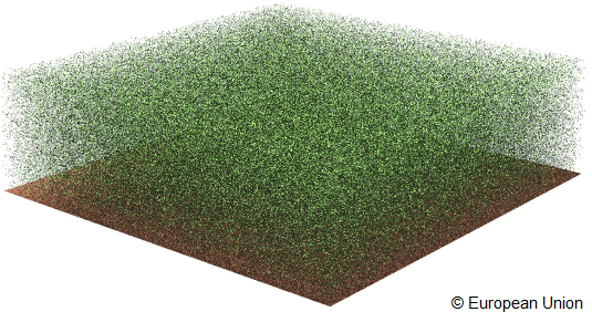
Graphical representation of Homogeneous Solar domain discrete scene.
Testcases
The tables below provide the details required to execute each of the experiments in this category. Every table is preceeded by the corresponding experiment identifier tag that is needed in the naming of the various measurement results files (see file naming and formatting conventions).
Results
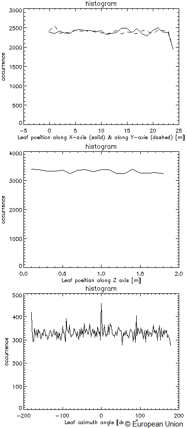
The first set of homogeneous discrete experiments refers to a vegetation canopy with a planophile leaf normal distribution and a scatterer radius of 0.1 m. An ASCII file with the radius (R), centre coordinates (Xc,Yc,Zc), and direction cosines (Dx,Dy,Dz) of every single leaf in a 25×25 m² canopy section can be found here. The file (is ~ 2.7 Mbytes and) contains 59683 lines of format R Xc Yc Zc Dx Dy Dz that may serve as input to your scene creation process (to save it you have to select the central frame of the web browser before saving its content). A resume of some statistical properties of the content of this ASCII file can be seen here:
The absence of any absolute "truth" renders the evaluation of RT models more tricky but, nevertheless, the model discernability issue can be addressed through the usage of "credible solutions". As a matter of fact, it can reasonably be admitted that the latter correspond to the actual values that could be measured from an instrument with its intrinsic limited accuracy.
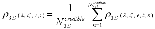
We attempted to examine the issue of model discernability by establishing, for all scenarios concerned, what could be considered as a "credible solution" by estimating the arithmetic mean of every BRF value calculated within a subset of the participating three-dimensional Monte Carlo model results.
Overall six different 3D MC models were allowed to contribute to the establishing of the ``credible'' solution. These are: DART, drat, FLIGHT, Rayspread, raytran, and sprint3. The following rules were applied when choosing the exact name and number of 3D MC models that then contributed to the establishing of the ``credible'' solution (note that both the name and number of 3D MC models may change between exeriments and also between individual measurement types, as outline in the table here):
Resume of some statistical properties of the content of this ASCII file.
For every RAMI BRF (flux) measurement, identify at least two (one) 3-D MC models that do not belone to the same RT modelling school/family,
If two models formt he same RT modellign school/family are available, e.g. raytran/Rayspread, choose the one with the least amount of apparent MC noise,
Remove all those 3D MC models from the reference set that are noticeably different from the main cluster of 3D MC models,
If sufficient models are contained in the main cluster of 3D MC simulations then remove those models that would introduce noticeable levels of MC noise into the reference set,
If there are two distinct cluster of 3D MC models, or no obvious cluster at all, then use all available 3D MC models to define a reference truth
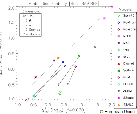
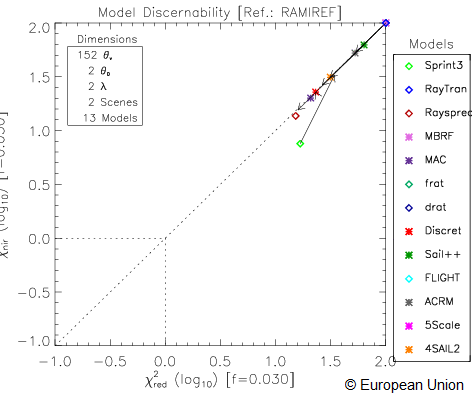
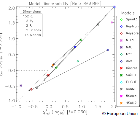
The figure displays the Chi-square metrics obtained in the red (x-axis) against those for the near-infrared (Y axis) using a value of 0.03 for the uncertainty f (equivalent to sensors having a 3% calibration accuracy).
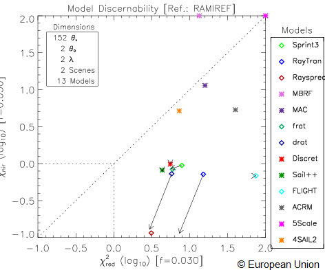
The figure displays the Chi-square metrics for single uncollided BRF components.
The figure displays the Chi-square metrics for single collided BRF components.
The figure displays the Chi-square metrics for multiple collided BRF components.
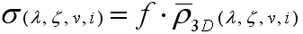
Once a suitable set of ``credible solutions'' are available the model discernability can then be analyzed by comparing the BRF values generated from individual models with those of the credible solution using a normalised Chi-square metric:
where the uncertainty estimator in the denominator (sigma) is simply expressed as a fraction of the credible BRF (at any given view angle).
The figure below displays the Chi-square metrics obtained in the red (x-axis) against those for the near-infrared (Y axis) using a value of 0.03 for the uncertainty f (equivalent to sensors having a 3% calibration accuracy):