
Phase: RAMI 3
The Spreading of Photons for Radiation INTerception (SPRINT) model was developed since it was felt that it would be desirable to have a model which can be used to realistically compute reflectance from a complex kilometer-level scene (consisting of different kinds of vegetation and non-vegetative elements) so that one can systematically study the effects of various parts of scenes and determine what aspects are important and how one can simplify the model to reduce the number of parameters, without losing the accuracy of the model. Also the model should be computationally very fast (a few minutes on a personal computer), requiring reasonable computer memory (less than a few hundred megabytes) and still incorporate heterogeneity in kilometer-level scenes.
The SPRINT model is capable to satisfy all these requirements.
It is universal in the sense that it can emulate turbid medium, geometrical, hybrid, and computer simulation models.
A part of the model is the generation of the kilometer-level scenes, which can contain various kinds of objects.
The computer time to calculate BRDF is a few minutes on a laptop computer, and is practically independent of the complexity of the scene. The basic model consists of several modules which are described separately:
This module allows a user to either interactively construct scenes and save them as data files for later use or input scene descriptions from data files. Scenes can be constructed by defining polygonal regions on an aerial map of a real scene and filling them with trees and other reflective objects (e.g., lakes, snow covered area, etc.). One can choose percentages of different types of trees in the polygonal region from an allowed set (See next subsection), and one can also choose their distributions.
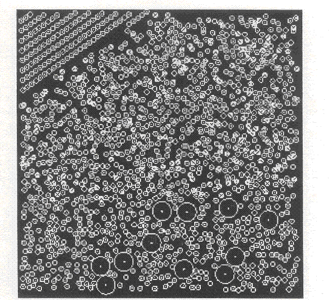
In the present implementation, trees from an allowed set of geometrical shapes can be placed in rows or distributed according to the Poisson or Neyman distribution (Chen and LeBlanc, 1997). Figure 1 shows a sample scene, with different distributions of trees in different areas. If desired, one can examine local regions in detail to see if the distribution of trees is as one had hoped. Figure 2 gives such details for a local region.
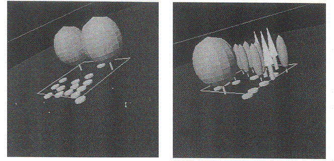
In the current implementation, a tree consists of a simple, geometrically shaped crown (ellipsoid, cylinder, cone, cylinder capped with a cone, or cube), with a cylindrical trunk. Inside the crown there is a turbid medium consisting of leaves and branches, each specified by density and angle distribution.
Trunks are treated as opaque geometrical objects. If desired, other objects can also be treated this way, e.g., the crown if one wants to emulate the geometrical models. Tree shapes can be allowed to overlap, or overlaps can be prohibited.
At present, leaves, branches, and soil are all treated as Lambertian scatterers, all specified by hemispherical reflectances and transmittances. (For soil and branches, transmittances are zero.) However, non-Lambertian scattering can be included. We should add that, in principle, one can make the scene as complex as one likes, although one may need extra computer memory to store the scene elements. For example, one can represent the tree or a plant by its detailed architecture, generated by an L-system or by a fractal based approach, as has been done in Goel et al. (1991).
The model uses ray-tracing/Monte Carlo methods, but what is different is the use of the concept of photon spreading to speed up the calculations of BRDF. As a photon passes through a scene, it collides with scene elements and is either reflected, transmitted or absorbed. An element can be either a real surface (trunks and soil) or a random variable (turbid media representing leaves, etc.).
The photon ends its trajectory by being absorbed by scene elements (including soil) or by being absorbed into the sky in a particular direction. BRDF is based on the total absorption of photons into the sky in specified viewing directions. BRDF is theoretically given by a limit of multiple integrals (a path integral) over potential photon collision points. This integral is approximated in the Monte Carlo method by generating a set of random paths.
In this method one needs to follow the movement of a photon as it moves through the canopy by scattering. In the photon spread method, random photon paths are also generated, but an integration over viewing directions is done at randomly chosen steps to assess the contribution of the photon towards the sky (and hence to BRDF) at that point. In effect, the photon partially spreads out as a continuous wave in a Lambertian fashion from the randomly chosen collision point (hence the term photon spread). In simple language, photon spread is like a flash bulb with light going in all directions.
If we imagine a photographic film in the viewing hemisphere, the BRDF is related to the picture made on the film from accumulated exposures by many flash bulbs, each corresponding to a photon spread.
If we imagine the film divided into a few pieces in directions of interest (viewing directions such as those for satellites), then the flash has to be considered only in those directions.
The BRDF is shown as a 3D plot which can be rotated, translated, and zoomed using the mouse to view from different angles and at different scales. We also calculate albedo and Fpar; see Thompson and Goel (2000) for details. To produce the hotspot, we used a version of the gap probability approach (see e.g., Qin et al., 1996 where various efforts to calculate hotspot are reviewed).
If it is known that a photon has traversed a given line segment without colliding with a scene element, then it follows that there must be no scene elements along that segment.
The probability distribution for the presence of scene elements near the segment therefore has to be modified to reflect this fact. This reduces the probability of collision for a photon that is nearly retracing its previous path after a collision. The hot-spot is simulated by introducing an estimate of this probability reduction. To some degree, the hotspot also arises from the geometry of real (as opposed to probabilistic) scene elements. This happens automatically. It should be added that to simulate the hotspot in a turbid medium of the kind inside each crown, a finite size is assumed for the scatterers, and a finite number of scatterers per unit volume is assumed.
The width of the hotspot depends on the size of the scatterers (which we take to be disks) and it goes to zero as the size of the scatterers goes to zero.